Table of contents

Introduction

In the interest of making data science processes accessible to non-specialists, I’ve written a collection of functions for doing a particularly common task in the exploratory phase of data analysis: the detection of outliers.

Why care about outliers? There are a couple of reasons:

1. Outliers distort the picture of the data we obtain using descriptive statitics and data visualization. When our goal is to understand the data, it is often worthwhile to disregard outliers.
2. Outliers play havoc with many machine learning algorithms and statistical models. When our goal is to predict, our models are often improved by ignoring outliers.
3. Outliers can be exactly what we want to learn about, especially for tasks like anomaly detection.

I’ll go through a few different ways of determining which observations in a dataset should be considered outliers, and when each is appropriate. The focus here is on repeatability. None of these recipes takes you from raw data to an analysis – they all assume that the relevant data has been extracted, and is in a sensible format. I define ‘sensible format’ as a Python list containing all the observations of the variable of interest. Note that the variable must be continuous, not categorical, for any of these functions to make sense.

A word of warning

None of these methods will deliver the objective truth about which of a dataset’s observations are outliers, simply because there is no objective way of knowing whether something is truly an outlier or an honest-to-goodness data point your model should account for. It is a decision you must make subjectively, depending on the goals of uour analysis. Nevertheless, there is some guidance to be found in the accumulated wisdom of the field: these functions are a great way to start wondering about which points in your data should be treated as outliers.

Methods

The three methods I’ll go through here are the Z-score method, and the modified Z-score method, and the IQR (interquartile range) method.

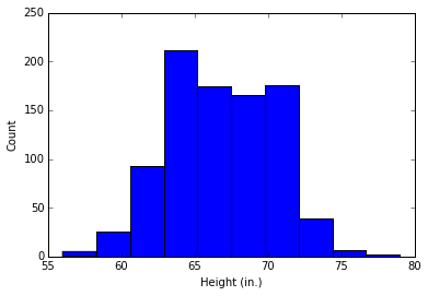
To show how the different methods work, I’ll make reference to an example dataset, Sir Francis Galton’s famous height dataset, made available by Random at the University of Alabama in Huntsville. The dataset records the heights of 898 people.

Here is a histogram showing the distribution of heights in the dataset:

Z-score method

The Z-score, or standard score, is a way of describing a data point in terms of its relationship to the mean and standard deviation of a group of points. Taking a Z-score is simply mapping the data onto a distribution whose mean is defined as 0 and whose standard deviation is defined as 1.

The goal of taking Z-scores is to remove the effects of the location and scale of the data, allowing different datasets to be compared directly. The intuition behind the Z-score method of outlier detection is that, once we’ve centred and rescaled the data, anything that is too far from zero (the threshold is usually a Z-score of 3 or -3) should be considered an outlier.

This function shows how the calculation is made:

import numpy as np

def outliers_z_score(ys):
    threshold = 3

    mean_y = np.mean(ys)
    stdev_y = np.std(ys)
    z_scores = [(y - mean_y) / stdev_y for y in ys]
    return np.where(np.abs(z_scores) > threshold)

The Z-score method relies on the mean and standard deviation of a group of data to measure central tendency and dispersion. This is troublesome, because the mean and standard deviation are highly affected by outliers – they are not robust. In fact, the skewing that outliers bring is one of the biggest reasons for finding and removing outliers from a dataset!

Modified Z-score method

Another drawback of the Z-score method is that it behaves strangely in small datasets – in fact, the Z-score method will never detect an outlier if the dataset has fewer than 12 items in it. This motivated the development of a modified Z-score method, which does not suffer from the same limitation.²

import numpy as np

def outliers_modified_z_score(ys):
    threshold = 3.5

    median_y = np.median(ys)
    median_absolute_deviation_y = np.median([np.abs(y - median_y) for y in ys])
    modified_z_scores = [0.6745 * (y - median_y) / median_absolute_deviation_y
                         for y in ys]
    return np.where(np.abs(modified_z_scores) > threshold)

A further benefit of the modified Z-score method is that it uses the median and MAD rather than the mean and standard deviation. The median and MAD are robust measures of central tendency and dispersion, respectively.

IQR method

Another robust method for labeling outliers is the IQR (interquartile range) method of outlier detection developed by John Tukey, the pioneer of exploratory data analysis. This was in the days of calculation and plotting by hand, so the datasets involved were typically small, and the emphasis was on understanding the story the data told. If you’ve seen a box-and-whisker plot (also a Tukey contribution), you’ve seen this method in action.¹

A box-and-whisker plot uses quartiles (points that divide the data into four groups of equal size) to plot the shape of the data. The box represents the 1st and 3rd quartiles, which are equal to the 25th and 75th percentiles. The line inside the box represents the 2nd quartile, which is the median.

The interquartile range, which gives this method of outlier detection its name, is the range between the first and the third quartiles (the edges of the box). Tukey considered any data point that fell outside of either 1.5 times the IQR below the first – or 1.5 times the IQR above the third – quartile to be “outside” or “far out”. In a classic box-and-whisker plot, the ‘whiskers’ extend up to the last data point that is not “outside”.

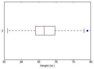
Let’s take the box-and-whisker plot above as an example. From the box, we can see that the median of the dataset falls at 66.5 inches, and that the first and third quartiles fall at approximately 64 and 70 inches, respectively. The whiskers show us that there are no outliers (as calculated by the IQR method) on the low end, but there is one on the high end, which is defined as over 78.25 inches.

To automate the process of finding outliers by the IQR method, you can use the following Python function:

import numpy as np

def outliers_iqr(ys):
    quartile_1, quartile_3 = np.percentile(ys, [25, 75])
    iqr = quartile_3 - quartile_1
    lower_bound = quartile_1 - (iqr * 1.5)
    upper_bound = quartile_3 + (iqr * 1.5)
    return np.where((ys > upper_bound) | (ys < lower_bound))

One benefit of using the interquartile range method is that, like the modified Z-score method, it uses a robust measure of dispersion.

Discussion

So, which method should you use? First, there is little harm in using all of them and seeing what picture emerges: in exploratory data analysis, there is no inference being made. There is therefore no increased risk of Type 1 error (false positives). That said, in my opinion, the Z-score method has the least to offer, because it is dependent on non-robust measures, and fails to report any outliers with low-size datasets.

Here are the results of running each of these functions on the Galton height data:

• Z-score: 56” (below); 78”, 79” (above)
• Modified Z-score: none
• IQR: 79” (above)

As you can see, no method is returning radically different results from any other. In a dataset with 898 observations, the difference between 0 and 3 outliers is not great.

One caveat: all of these methods will encounter problems with a strongly skewed dataset. If the data is distributed in a strongly asymmetrical fashion, it will need to be re-expressed before applying any of these methods.

Conclusion

It is important to reiterate that these methods should not be used mechanically. They should be used to explore the data – they let you know which points might be worth a closer look. What to do with this information depends heavily on the situation. Sometimes it is appropriate to exclude outliers from a dataset to make a model trained on that dataset more predictive. Sometimes, however, the presence of outliers is a warning sign that the real-world process generating the data is more complicated than expected.

As an astute commenter on CrossValidated put it: “Sometimes outliers are bad data, and should be excluded, such as typos. Sometimes they are Wayne Gretzky or Michael Jordan, and should be kept.” Domain knowledge and practical wisdom are the only ways to tell the difference.